Basics in R
Last updated:
Disclaimer:
I never took a formal CS course so my terminology and explanations of concepts may be questionable at times.
Tip:
Google is your friend. 99% of coding relies on if you can Google the right question into the search bar. I recommend going to Stack Overflow and other forums to look for answers. The other 1% relies on whether you can interpret the answer and modify it to fit your needs.
Installation
-
Install R by going to CRAN which you can access by clicking here. Find a URL which is closest to you (for Pittsburgh people, this will be Statlib, Carnegie Mellon University). Click on the Download link to whichever operating system you’re working in (Linux, macOS, or Windows) and follow the directions.
-
Windows: click on the hyperlink, “install R for the first time” and then click the download R link.
-
macOS: this is a bit trickier and will heavily depend on whether you have Intel or the Apple Silicon processor. More details below…
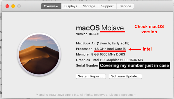
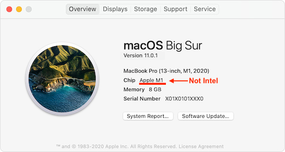
For macOS users, you need to check which version of macOS you’re running on and also which processor (i.e. Intel or Apple silicon). You can check this by clicking on the apple icon on the top left of your screen, and selecting About This Mac from the dropdown menu.
If you are using an older version of the macOS (i.e. Intel based), then next to Processor, it should say Intel:
If you are using the newer Apple M1 macbooks which uses Apple silicon, then next to Chip, it should say Apple M1 instead of Intel:
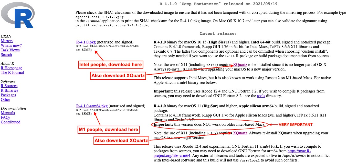
If you are using Intel on a macOS version that is 10.9 (i.e. Mavericks) or later, then you need to also install XQuartz. Then you will install R-4.1.0.pkg and NOT the R-4.1.0-arm64.pkg.
If you are using Apple M1 on a macOS version that is 11.0 (i.e. Big Sur) or later, then you need to install R-4.1.0-arm64.pkg. You may still need to install XQuartz. Important: This package will not work if your processor is Intel based!!!
-
-
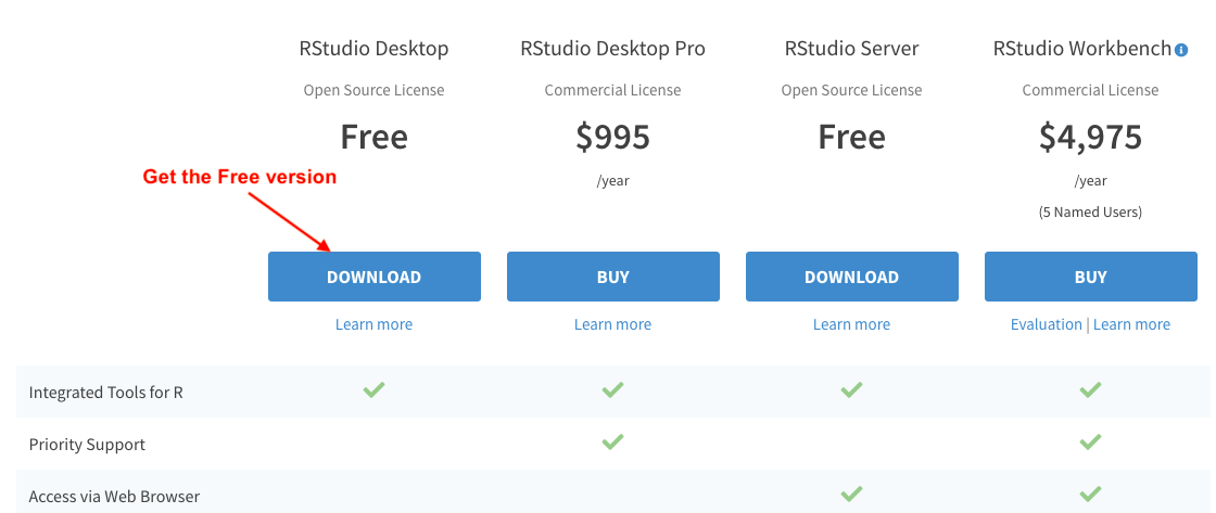
Download the free version of RStudio Desktop. This is an Integrated Development Environment (IDE) where you will write your code. You can technically write directly in R instead of RStudio but for the sake of making your life easier, please don’t do this. The free version works fine for our purpose.
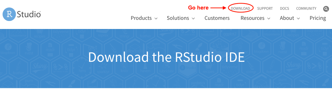
After you get to the Download page, scroll down until you see the free download version and click DOWNLOAD. Or alternatively, go here.
-
Run line-by-line by pressing Cmd+Enter or Ctrl+Enter.
-
Eventually, after a couple of months/years of using R you may get updates for R, for the packages that you have installed in R, or even for your operating system. Beware when you update anything (this includes big Windows and macOS updates). Some things may be dependent on other packages or may work only on certain versions of R or operating systems, and they could potentially stop cooperating if you update things. Just double check and make sure you can revert to an old version should things go south.
RStudio Basics
Intoduction
When you first open RStudio, you will get 4 panels and each panel will have a different purpose. Don’t worry if you only see 3 panels–you may just need to open an R script file which will be covered later.
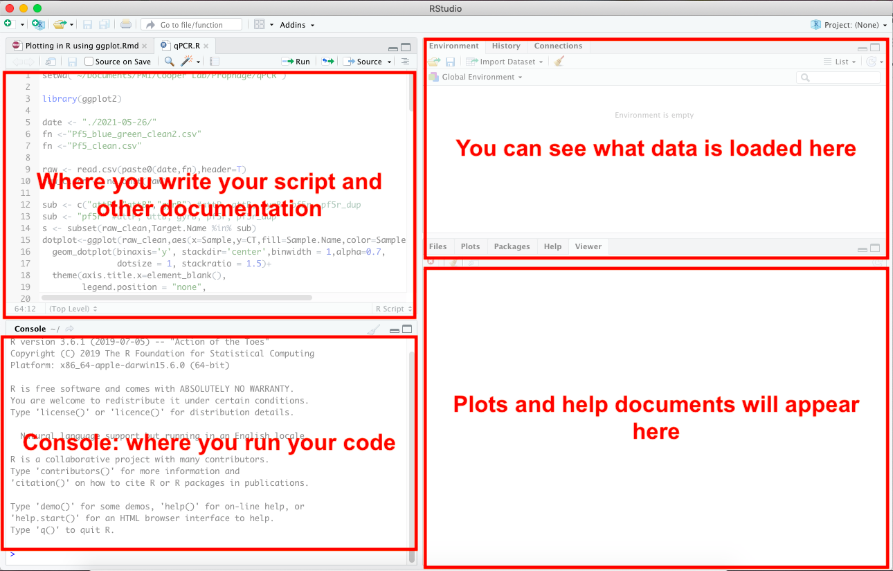
Top left panel: This is where you will write your code. Think of it like a Word document. Once you write your line of code, you can press Cmd+Enter (or Ctrl+Enter) to run a single line of code.
Bottom left panel: This is your console. You can technically write your code directly in here but since you’ll eventually want to save your code, try to write it in the top left panel.
Top right panel: You will see all of the variables that you have named and data that you have loaded here. You don’t need to worry about this at the moment.
Bottom right panel: This is where your plots will appear if you plotted data. You can also read the help documentation from here by using the help( ) function or writing a ? (question mark) before the function to learn more about that function. I will explain this is in the 2.5 Getting help section.
Open a new document
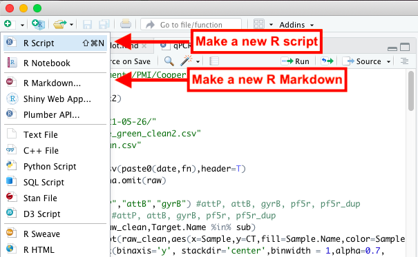
There are two types of documents that will be of useful for you. For the sake of this tutorial, you can focus on R script files for now. R script files are good for writing just code and a few comments here and there. If you are feeling more advanced, you can use the R markdown document. This is more useful if you want to write notes down and keep track of what you did kind of like a lab notebook.
Open a new R Script document by going to File -> New File -> R Script, or you can press on the top right button with the green plus sign and click R Script from the dropdown menu (as seen in the picture below).
Installing and loading packages
Installing packages only needs to be done once. Once you have installed a package, all you need to do is load the package everytime you need to use it in a new R session.
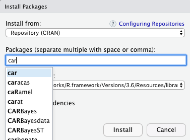
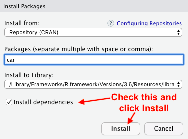
This step is for users installing the package, car, for the first time and this only needs to be done once.
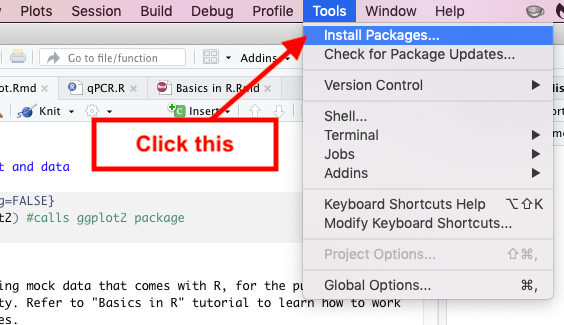
Go to Tools located at the top and click Install Packages. Then under the Packages search bar search for “car” and select car once it comes up. Then check off Install dependencies and click Install.
You only need to install a particular package once. Once you do, every time you have a new R session, you must load that package so that R can access it by using the following function:
library(car)
Set your working directory
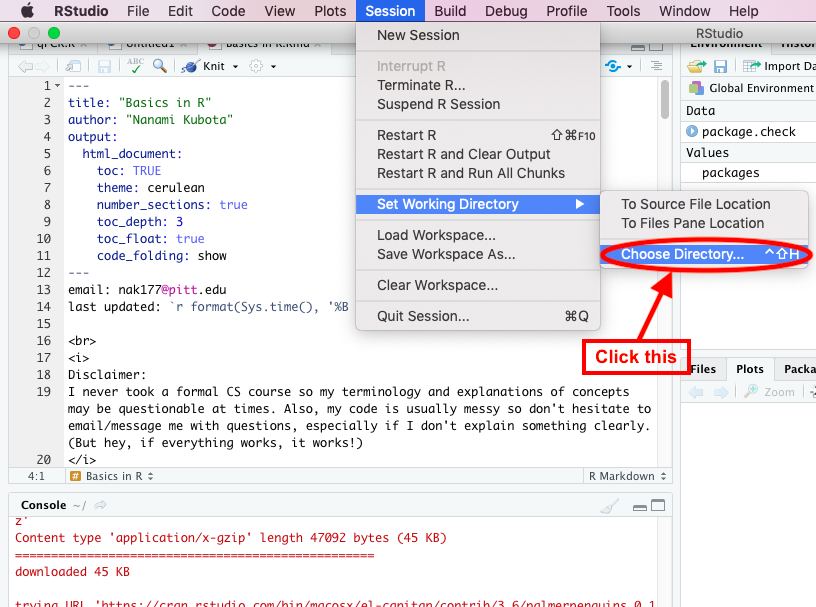
Always begin by setting your working directory. The directory is the location of the folder where you would like to work from. Generally, you will have you data, plots, and R script within this folder to work from. You can do this manually by going to the top menu bar and click Session -> Set Working Directory -> Choose Directory….
Your life will be easier if you copy/paste the line of code that is generated in the console after this and incorporate it into your script for future reference. That way you can just press Cmd+Enter to set your working directory everytime you need to run some code, instead of manually entering it each time via the dropdown menu. The below is my working directory and this will be different for every person:
setwd("~/Documents/PMI/Cooper Lab/CS tutorial/tutorial")
Functions
A function is a command that you write and run so that R can do that command on another object. For example, in the previous section we manually set the working directory, which produced a line of code using the setwd( ) function. Using the setwd( ) function, we are able to set the working directory to our folder of choice by writing the file path to that folder. In my example, my file path is “~/Documents/PMI/Cooper Lab/CS tutorial/tutorial”.
Usually, functions are written in the following format:
function(x)
Where x is the object you would like to pass through the function. The above example is a very simple one, and some functions can require you to pass multiple objects through it. In order to know what you need to enter within the paranthesis, I recommend that you look at the documentation for the function or look up examples on how to use the function online. We will cover how to look at documentation for functions in the next section.
Getting help
As you start to use different functions, you may want to look at the documentation on that function in case you get stuck or need to learn more about a particular function.
Let’s say you want to learn more about the plot( ) function. You can look at the documentation for plot( ) by doing the following:
help("plot")
An alternative to this (which I prefer since it’s faster to type out) is:
?plot
Adding comments
In an R script, anything after the # mark in a line of code will be considered a comment (a string of characters that R ignores). Not adding the # when you write a comment can give you an error since R will think it’s part of the code and try to run it.
Writing comments are helpful especially if you want to be able to look back at your script and know the purpose of each line of code. It is also helpful for anyone who needs to use and understand your script. To write a comment:
#This is how to write a proper comment
If you are using R markdown, you do not need to use # to write comments unless you plan to write comments inside a code block (which you can produce by pressing Cmd+Alt+I). Ignore this if you are using R Script.
Calculations
Arithmetic
You can use R as a calculator. Notations to enter your calculations are as follows:
1+2 #should give you 3
1-2 #should give you -1
2*3 #should give you 6
100/25 #should give you 4
Log, square root, power
R can also do more complex calculations:
log(2) #log of 2 equals 0.6931472
sqrt(9) #square root of 9 equals 3
10^1 #power of 10 to the 1 is 10
Variable names and values
You can assign values (numbers, characters, logical values, etc.) to variables. Make sure the variable name does not contain any spaces. The only acceptable special symbols are the underscore (_) and period (.). Also, try to make sure your variable name doesn’t start with a number, and that the name doesn’t consist of just number(s):
hours_slept <- 3 #this assigns the value 3 onto "hours_slept"
student_name <- "Nanami" #you can also assign characters but characters must be in quotation marks
is.awake.in.class <- FALSE #can do TRUE or FALSE. Must be all caps and no quotation marks.
is.awake.in.class <- F #using T or F also works too. Don't use quotation marks.
is.awake.in.class #should return FALSE
Variables can have multiple values too. Use c( ) to bind together multiple values:
bad_at <- c("staying awake", "paying attention", "time management")
time_awake <- c(5,7,6,9,7)
Asking true or false
Logical operators
You can ask R to determine whether a condition is true or false:
student_name == "Nanami" #ask if student_name is "Nanami"
is.awake.in.class == TRUE #ask if is.awake.in.class equals TRUE. Should return FALSE.
hours_slept > 3 #ask if hours_slept is greater than 3
hours_slept < 3 #ask if hours_slept is less than 3
hours_slept >= 3 #ask if hours_slept is greater than or equal to 3
hours_slept <= 3 #ask if hours_slept is less than or equal to 3
Dealing with a list or larger variable
Let’s say you have a list of variables (e.g. time_awake variable from a previous section), and you want to see if a certain number or character is included within the list (e.g. the number 9). There are two ways to go about this, and they are slightly different from each other.
The first way is to check each element in a list and return a TRUE or FALSE for EVERY element in a list:
time_awake == 9 #asks if each element in time_awake (i.e. 5, 7, 6, 9, 7) is the number 9; it should check each number return a TRUE or FALSE for EVERY number in the list
## [1] FALSE FALSE FALSE TRUE FALSE
time_awake != 9 #asks if each element is NOT the number 9 and returns TRUE or FALSE for EVERY number in the list
## [1] TRUE TRUE TRUE FALSE TRUE
The second way is to check the list as a whole and return a TRUE or FALSE just once to tell you if the list includes what you are looking for:
9 %in% time_awake #ask if 9 is even present in time_awake AT ALL; should return just TRUE since it is check a list as a whole
## [1] TRUE
!(9 %in% time_awake) #ask if 9 is NOT in time_awake; should return just FALSE
## [1] FALSE
Although at first glance both methods seem to do the same things, this nuance will become important once you start using larger datasets. For example, if you have 1000 numbers in a list and you want to see if the number 99 appears even once in the list, you don’t want to do the first method since it will give you a TRUE or FALSE for every number in the list. Instead, you will go with the second method.
Working with data
R has many datasets that come with the program so that you can have mock data to play around with. The type of data we will be working with is called data frame. A data frame is a 2-dimensional table-like structure with columns and rows. Let’s try loading a data frame on flower measurements:
library(datasets) #load dataset package
data(iris) #load dataset called "iris"
head(iris) #shows only the first few rows of the "iris" data.frame
##   Sepal.Length Sepal.Width Petal.Length Petal.Width Species
## 1          5.1         3.5          1.4         0.2  setosa
## 2          4.9         3.0          1.4         0.2  setosa
## 3          4.7         3.2          1.3         0.2  setosa
## 4          4.6         3.1          1.5         0.2  setosa
## 5          5.0         3.6          1.4         0.2  setosa
## 6          5.4         3.9          1.7         0.4  setosa
You can see that the data frame contains 5 columns. Since we used the head( ) function, we only see the first few rows. It is always a good idea to use head( ) when viewing large data frames since data frames can potentially have many rows and columns.
See how the computer will try to show you everything if you just enter iris:
iris
Checking dataset dimensions and summary of data
To check the dimensions of the data frame without having to look at the whole data frame use:
nrow(iris) #shows number of rows. It should say 150.
## [1] 150
ncol(iris) #shows number of columns. It should say 5.
## [1] 5
dim(iris) #shows dimension. 150 rows by 5 columns.
## [1] 150 5
To see a general summary of your data, you can do:
summary(iris)
##   Sepal.Length    Sepal.Width     Petal.Length    Petal.Width
##  Min.   :4.300   Min.   :2.000   Min.   :1.000   Min.   :0.100
##  1st Qu.:5.100   1st Qu.:2.800   1st Qu.:1.600   1st Qu.:0.300
##  Median :5.800   Median :3.000   Median :4.350   Median :1.300
##  Mean   :5.843   Mean   :3.057   Mean   :3.758   Mean   :1.199
##  3rd Qu.:6.400   3rd Qu.:3.300   3rd Qu.:5.100   3rd Qu.:1.800
##  Max.   :7.900   Max.   :4.400   Max.   :6.900   Max.   :2.500
##        Species
##  setosa    :50
##  versicolor:50
##  virginica :50
##
##
##
Subgroups/Columns in datasets
To look at subgroups within your data, you can do:
ls(iris) #ls() lists subgroups alphabetically and NOT by column order.
## [1] "Petal.Length" "Petal.Width" "Sepal.Length" "Sepal.Width" "Species"
Then to look at just the values within a subgroup, you can do:
iris$Sepal.Length
##   [1] 5.1 4.9 4.7 4.6 5.0 5.4 4.6 5.0 4.4 4.9 5.4 4.8 4.8 4.3 5.8 5.7 5.4 5.1
##  [19] 5.7 5.1 5.4 5.1 4.6 5.1 4.8 5.0 5.0 5.2 5.2 4.7 4.8 5.4 5.2 5.5 4.9 5.0
##  [37] 5.5 4.9 4.4 5.1 5.0 4.5 4.4 5.0 5.1 4.8 5.1 4.6 5.3 5.0 7.0 6.4 6.9 5.5
##  [55] 6.5 5.7 6.3 4.9 6.6 5.2 5.0 5.9 6.0 6.1 5.6 6.7 5.6 5.8 6.2 5.6 5.9 6.1
##  [73] 6.3 6.1 6.4 6.6 6.8 6.7 6.0 5.7 5.5 5.5 5.8 6.0 5.4 6.0 6.7 6.3 5.6 5.5
##  [91] 5.5 6.1 5.8 5.0 5.6 5.7 5.7 6.2 5.1 5.7 6.3 5.8 7.1 6.3 6.5 7.6 4.9 7.3
## [109] 6.7 7.2 6.5 6.4 6.8 5.7 5.8 6.4 6.5 7.7 7.7 6.0 6.9 5.6 7.7 6.3 6.7 7.2
## [127] 6.2 6.1 6.4 7.2 7.4 7.9 6.4 6.3 6.1 7.7 6.3 6.4 6.0 6.9 6.7 6.9 5.8 6.8
## [145] 6.7 6.7 6.3 6.5 6.2 5.9
There are other ways to look at the values within a subgroup. If your dataset is a table format, you can enter the row number to get information on specific cell(s) within a table:
iris[2,] #get all the values in row #2 from all subgroups; the first number in [ ] denotes the row number; don't forget the comma
##   Sepal.Length Sepal.Width Petal.Length Petal.Width Species
## 2          4.9           3          1.4         0.2  setosa
For columns, it is the same concept as the above but can be a bit tricky to wrap your head around. You will first want to know which column number (first, second, third, etc.) your subgroup of interest is. To do this use colnames( ) which is DIFFERENT from the ls( ) function since it will list column name by column order and not alphabetically:
colnames(iris) #get the list of column names in iris by column order and not alphabetically
## [1] "Sepal.Length" "Sepal.Width" "Petal.Length" "Petal.Width" "Species"
Let’s say we are interested in the subgroup, Petal.Length. You can use iris$Petal.Length to do the following but you can also call this by column number/order. This is useful when you don’t want to type out the column name to call your subgroup of interest.
Since Petal.Length is listed third in the previous colnames( ) function, we can do the following to get the values within Petal.Length:
iris[,3] #get the values under the Petal.Length subgroup; equivalent of iris$Petal.Length; the second number in [ ] denotes the column number; don't forget the comma
##   [1] 1.4 1.4 1.3 1.5 1.4 1.7 1.4 1.5 1.4 1.5 1.5 1.6 1.4 1.1 1.2 1.5 1.3 1.4
##  [19] 1.7 1.5 1.7 1.5 1.0 1.7 1.9 1.6 1.6 1.5 1.4 1.6 1.6 1.5 1.5 1.4 1.5 1.2
##  [37] 1.3 1.4 1.3 1.5 1.3 1.3 1.3 1.6 1.9 1.4 1.6 1.4 1.5 1.4 4.7 4.5 4.9 4.0
##  [55] 4.6 4.5 4.7 3.3 4.6 3.9 3.5 4.2 4.0 4.7 3.6 4.4 4.5 4.1 4.5 3.9 4.8 4.0
##  [73] 4.9 4.7 4.3 4.4 4.8 5.0 4.5 3.5 3.8 3.7 3.9 5.1 4.5 4.5 4.7 4.4 4.1 4.0
##  [91] 4.4 4.6 4.0 3.3 4.2 4.2 4.2 4.3 3.0 4.1 6.0 5.1 5.9 5.6 5.8 6.6 4.5 6.3
## [109] 5.8 6.1 5.1 5.3 5.5 5.0 5.1 5.3 5.5 6.7 6.9 5.0 5.7 4.9 6.7 4.9 5.7 6.0
## [127] 4.8 4.9 5.6 5.8 6.1 6.4 5.6 5.1 5.6 6.1 5.6 5.5 4.8 5.4 5.6 5.1 5.1 5.9
## [145] 5.7 5.2 5.0 5.2 5.4 5.1
Character variables within subgroups
Sometimes, the variable contains names or characters instead of numerical data (like the list of Species in iris). Instead of looking at each plant sample’s species name (since there are some plant samples that are from the same species), you can just get a list of all the species names present in the list by using the function, levels( ):
levels(iris$Species)
## [1] "setosa" "versicolor" "virginica"
See how much more cleaner levels( ) is rather than doing iris$Species:
iris$Species
Dealing with missing data (NAs)
Some data can have NA in the dataset, which means there is a missing value or no value assigned there. Let’s make an example dataset with NA by replacing a value in iris$Sepal.Length with NA:
mock <- iris #it is always a good idea to make a new variable which is a duplicate of your data in order to avoid overwriting it by accident
mock$Sepal.Length[3] <- NA #replace the 3rd element with NA
mock$Sepal.Length #you can see that the 3rd element is now NA
##   [1] 5.1 4.9  NA 4.6 5.0 5.4 4.6 5.0 4.4 4.9 5.4 4.8 4.8 4.3 5.8 5.7 5.4 5.1
##  [19] 5.7 5.1 5.4 5.1 4.6 5.1 4.8 5.0 5.0 5.2 5.2 4.7 4.8 5.4 5.2 5.5 4.9 5.0
##  [37] 5.5 4.9 4.4 5.1 5.0 4.5 4.4 5.0 5.1 4.8 5.1 4.6 5.3 5.0 7.0 6.4 6.9 5.5
##  [55] 6.5 5.7 6.3 4.9 6.6 5.2 5.0 5.9 6.0 6.1 5.6 6.7 5.6 5.8 6.2 5.6 5.9 6.1
##  [73] 6.3 6.1 6.4 6.6 6.8 6.7 6.0 5.7 5.5 5.5 5.8 6.0 5.4 6.0 6.7 6.3 5.6 5.5
##  [91] 5.5 6.1 5.8 5.0 5.6 5.7 5.7 6.2 5.1 5.7 6.3 5.8 7.1 6.3 6.5 7.6 4.9 7.3
## [109] 6.7 7.2 6.5 6.4 6.8 5.7 5.8 6.4 6.5 7.7 7.7 6.0 6.9 5.6 7.7 6.3 6.7 7.2
## [127] 6.2 6.1 6.4 7.2 7.4 7.9 6.4 6.3 6.1 7.7 6.3 6.4 6.0 6.9 6.7 6.9 5.8 6.8
## [145] 6.7 6.7 6.3 6.5 6.2 5.9
Sometimes you do not want NA in your dataset when doing calculations, or when plotting. To get rid of NA, you can:
clean <- na.omit(mock$Sepal.Length) #omit NA from mock$Sepal.Length
clean
##   [1] 5.1 4.9 4.6 5.0 5.4 4.6 5.0 4.4 4.9 5.4 4.8 4.8 4.3 5.8 5.7 5.4 5.1 5.7
##  [19] 5.1 5.4 5.1 4.6 5.1 4.8 5.0 5.0 5.2 5.2 4.7 4.8 5.4 5.2 5.5 4.9 5.0 5.5
##  [37] 4.9 4.4 5.1 5.0 4.5 4.4 5.0 5.1 4.8 5.1 4.6 5.3 5.0 7.0 6.4 6.9 5.5 6.5
##  [55] 5.7 6.3 4.9 6.6 5.2 5.0 5.9 6.0 6.1 5.6 6.7 5.6 5.8 6.2 5.6 5.9 6.1 6.3
##  [73] 6.1 6.4 6.6 6.8 6.7 6.0 5.7 5.5 5.5 5.8 6.0 5.4 6.0 6.7 6.3 5.6 5.5 5.5
##  [91] 6.1 5.8 5.0 5.6 5.7 5.7 6.2 5.1 5.7 6.3 5.8 7.1 6.3 6.5 7.6 4.9 7.3 6.7
## [109] 7.2 6.5 6.4 6.8 5.7 5.8 6.4 6.5 7.7 7.7 6.0 6.9 5.6 7.7 6.3 6.7 7.2 6.2
## [127] 6.1 6.4 7.2 7.4 7.9 6.4 6.3 6.1 7.7 6.3 6.4 6.0 6.9 6.7 6.9 5.8 6.8 6.7
## [145] 6.7 6.3 6.5 6.2 5.9
## attr(,"na.action")
## [1] 3
## attr(,"class")
## [1] "omit"
Note: We assigned a new variable, clean, which is the same as mock$Sepal.length but has NA omitted. This does not mean the original variable mock and its subgroup, Sepal.Length, has NA omitted:
mock$Sepal.Length
##   [1] 5.1 4.9  NA 4.6 5.0 5.4 4.6 5.0 4.4 4.9 5.4 4.8 4.8 4.3 5.8 5.7 5.4 5.1
##  [19] 5.7 5.1 5.4 5.1 4.6 5.1 4.8 5.0 5.0 5.2 5.2 4.7 4.8 5.4 5.2 5.5 4.9 5.0
##  [37] 5.5 4.9 4.4 5.1 5.0 4.5 4.4 5.0 5.1 4.8 5.1 4.6 5.3 5.0 7.0 6.4 6.9 5.5
##  [55] 6.5 5.7 6.3 4.9 6.6 5.2 5.0 5.9 6.0 6.1 5.6 6.7 5.6 5.8 6.2 5.6 5.9 6.1
##  [73] 6.3 6.1 6.4 6.6 6.8 6.7 6.0 5.7 5.5 5.5 5.8 6.0 5.4 6.0 6.7 6.3 5.6 5.5
##  [91] 5.5 6.1 5.8 5.0 5.6 5.7 5.7 6.2 5.1 5.7 6.3 5.8 7.1 6.3 6.5 7.6 4.9 7.3
## [109] 6.7 7.2 6.5 6.4 6.8 5.7 5.8 6.4 6.5 7.7 7.7 6.0 6.9 5.6 7.7 6.3 6.7 7.2
## [127] 6.2 6.1 6.4 7.2 7.4 7.9 6.4 6.3 6.1 7.7 6.3 6.4 6.0 6.9 6.7 6.9 5.8 6.8
## [145] 6.7 6.7 6.3 6.5 6.2 5.9