Mapping in R
Last updated:
Prepare your data
You will need the following packages:
library(sf)
library(ggplot2)
library(RColorBrewer)
library(plyr)
library(tibble)
library(grid)
Look up appropriate EPSG code for the region you want to map at https://epsg.io/
For this example, we will be using EPSG:2263 and plotting New York City school district borders as well as the locations of various NYC high schools.
To view information for EPSG:2263, run:
st_crs("EPSG:2263")
Get shapefile from NYC OpenData. The school district shapefile data can be found here: [https://data.cityofnewyork.us/Education/School-Districts/r8nu-ymqj]
Click on the “Export” tab and under “Download Geospatial Data”, click the “Shapefile” hyperlink. This should prompt a download.
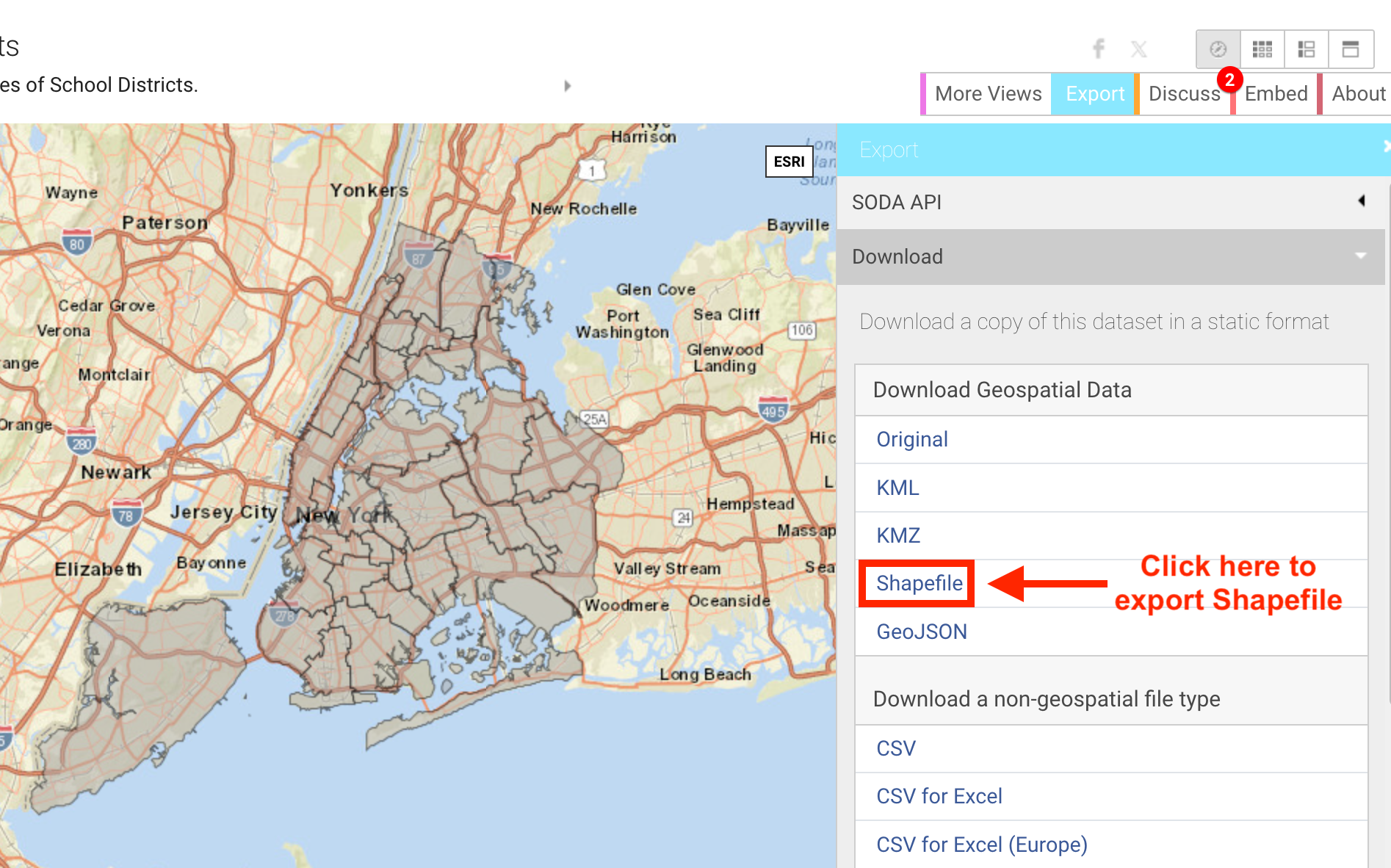
Unzip the file and you should have a folder with multiple files inside.
Next we will read the map:
school <- st_read("./data/School Districts")
Plot in ggplot
We will use the RColorBrewer to get our color codes for the 32 school districts.
bp <- brewer.pal(5, "RdYlBu") #get 5 colors from the RdYlBu palette
col <- colorRampPalette(bp) #generates function to create more colors from bp
mycolors <- sample(col(32)) #generate 32 colors and randomly reorder the color codes
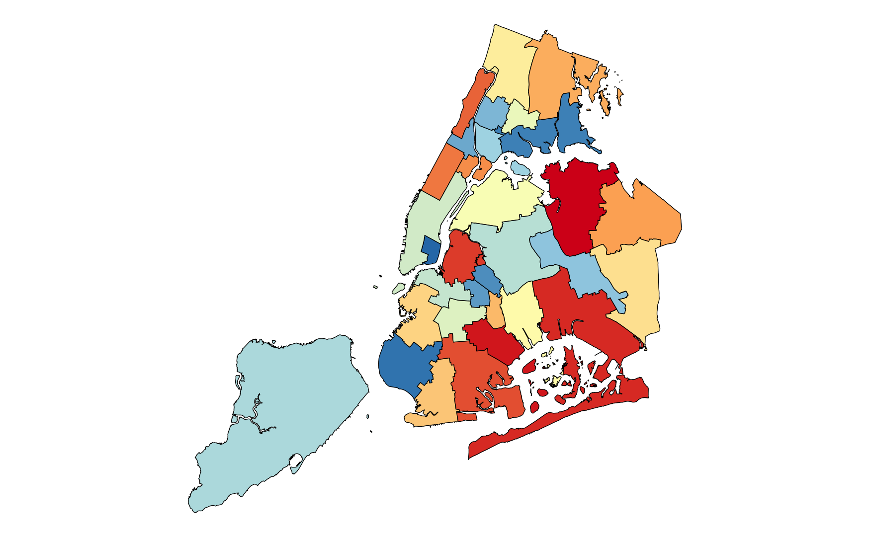
Then use ggplot to plot the map and color by school district:
school_map <- ggplot(data=school_sp, aes(fill=as.factor(school_dis)))+
  geom_sf(color="black",show.legend = FALSE)+
  scale_fill_manual(values = mycolors)+
  theme_void()
school_map
Your map should look like this (the colors might be slightly different depending on how the color order was randomized):
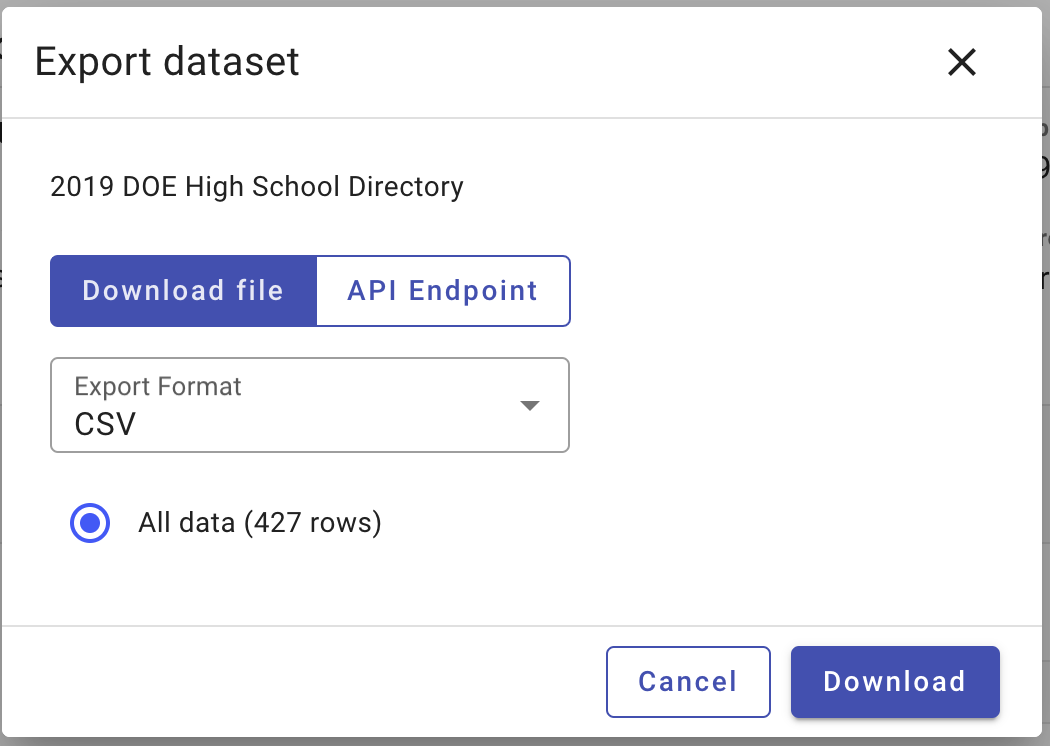
Lets plot all the high schools onto the map. Download the csv file from: [https://data.cityofnewyork.us/Education/2019-DOE-High-School-Directory/uq7m-95z8/about_data]
To export the data, click the “Export” button and export all the data as a csv file.
Lets read the csv file into R as a dataframe. Since there are many columns, we will select only those that we are interested in (i.e. Latitude and Longitude column):
hs <- read.csv("./data/2019_DOE_High_School_Directory_20240207.csv") %>%
  select(Latitude,Longitude)
Use the st_as_sf() function to convert the dataframe into a shapefile (sf) object.
hs_sp <- st_as_sf(hs,coords = c("Longitude","Latitude"), crs="+proj=longlat +datum=WGS84") #tell R to look at the columns named "Longitude" and "Latitude" for the longitude and latitude. Note that the order of calling "Longitude" before "Latitude" matters
Create a new object that only contains the geometry value of the shapefile.
clean_hs <- hs_sp %>%
  select(geometry)
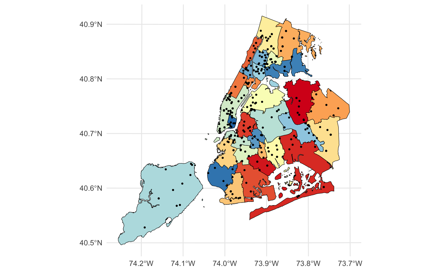
Plot using ggplot:
hs_map <- ggplot()+
  geom_sf(data=school_sp,aes(fill=as.factor(school_dis)),color="black",show.legend = FALSE)+
  scale_fill_manual(values = mycolors)+
  geom_sf(data=clean_hs, color="black", size=0.5)+
  theme_minimal()
hs_map
Your map should look like this: